门控循环单元 (GRU)
1. 核心概念与代码映射
1.1 门控循环单元 (GRU)
代码实现:EfficientGRU类中的torch.nn.GRU层
- 核心机制:GRU通过更新门和重置门控制信息的流动。更新门控制当前输入和过去状态的比例,而重置门则决定过去状态在当前计算中的影响。这使得GRU能够有效地捕捉长期依赖关系,且避免梯度消失问题
- 代码参数:
- SMOTE 过采样(
load_data函数):
用SMOTE(Synthetic Minority Over-sampling Technique)生成新样本以增强某一类别的样本量if smote_available:
smote = SMOTE(sampling_strategy='minority', random_state=42)
X, y = smote.fit_resample(X, y) - 类别权重计算:通过
calculate_class_weights生成权重向量,传入CrossEntropyLoss(代码中隐含实现)。1.3 特征工程技术
- 方差阈值筛选(
load_data函数):
移除低方差特征,以减少噪声和过拟合from sklearn.feature_selection import VarianceThreshold
selector = VarianceThreshold(threshold=0.1)
X = selector.fit_transform(X) - 随机森林特征选择(
select_important_features函数):基于随机森林feature_importances_筛选前 54 个重要特征,代码如下:def select_important_features(X, y, n_features=54):
model = RandomForestClassifier(n_estimators=100, random_state=42)
model.fit(X, y)
importances = model.feature_importances_
indices = np.argsort(importances)[::-1]
return X[:, indices[:n_features]]2. 模型架构详解(代码逐行解析)
2.1 网络结构定义
- GRU层:使用PyTorch提供的
torch.nn.GRU创建一个门控循环单元(GRU)层。- `input_dim`是输入特征的维度。 - `hidden_dim`(默认128)是GRU单元的隐藏层维度。 - `num_layers`表示层数,设置为2表示构建两层的GRU。 - `batch_first=True`确保输入数据的第一维表示批次大小,这在处理时序数据时更为直观。 - `bidirectional=False`表示该GRU层是单向的(如果设置为`True`则代表双向GRU)。 - `dropout=dropout`用于在层之间应用Dropout,以减轻过拟合。 - 全连接层与Dropout:
self.fc1 = torch.nn.Linear(hidden_dim, 256)定义了一个从隐藏层到256维的全连接层。self.dropout = torch.nn.Dropout(dropout)应用Dropout,以防止模型过拟合。self.fc2 = torch.nn.Linear(256, output_dim)定义了一个从256维到输出维度的全连接层,output_dim是任务的类别数,这里设为7。
- -
forward方法定义了模型的前向传播过程:h0:初始化隐状态为零,形状为(num_layers, batch_size, hidden_dim)。这个状态用于GRU单位,存储之前时刻的隐状态。out, _ = self.gru(x, h0):将输入x和初始化的隐状态h0传入GRU层,输出为out,形状为(batch_size, seq_len, hidden_dim)。- 在单时间步的情况下(例如,
seq_len=1),out的形状相当于(batch_size, 1, hidden_dim)。
- 在单时间步的情况下(例如,
out = torch.mean(out, dim=1):对时间维度进行平均池化。对于单时间步输入,这一步可以视作直接提取特征,而因GRU的输出序列在这里只包含一个时间步。out = self.fc1(out):将池化后的输出传递给全连接层fc1。out = torch.relu(out):在全连接层之后使用ReLU激活函数引入非线性。out = self.dropout(out):将Dropout应用于该层输出。out = self.fc2(out):将结果传递至最后的全连接层获得输出。return out:返回模型预测的输出。class EfficientGRU(torch.nn.Module):
def __init__(self, input_dim, hidden_dim=128, num_layers=2, output_dim=7, dropout=0.2):
super().__init__()
# GRU层:2层,隐藏维度128,启用Dropout
self.gru = torch.nn.GRU(
input_dim, hidden_dim, num_layers=num_layers,
batch_first=True, bidirectional=False, dropout=dropout
)
# 全连接层 + Dropout
self.fc1 = torch.nn.Linear(hidden_dim, 256)
self.dropout = torch.nn.Dropout(dropout)
self.fc2 = torch.nn.Linear(256, output_dim)
def forward(self, x):
h0 = torch.zeros(self.gru.num_layers, x.size(0), self.gru.hidden_size).to(x.device)
out, _ = self.gru(x, h0) # (batch_size, 1, hidden_dim)(单时间步)
out = torch.mean(out, dim=1) # 时间维度平均池化
out = self.fc1(out)
out = torch.relu(out)
out = self.dropout(out)
out = self.fc2(out)
return out
2.2 关键设计点
- 单时间步适配:通过
unsqueeze(1)为静态特征添加seq_len=1(代码中preprocess_data函数实现)。 - 池化简化:因单时间步,
torch.mean(out, dim=1)等价于直接提取特征,简化时序处理。3. 数据处理全流程代码解析
3.1 数据加载与清洗(
load_data函数)def load_data(file_path):
data = pd.read_csv(file_path)
X = data.drop('Cover_Type', axis=1)
y = data['Cover_Type']
# 移除低方差特征
selector = VarianceThreshold(threshold=0.1)
X = selector.fit_transform(X)
# SMOTE过采样(若已安装imblearn)
if smote_available:
    smote = SMOTE(sampling_strategy='minority', random_state=42)
    X, y = smote.fit_resample(X, y)
return X, y3.2 数据集划分与预处理(
preprocess_data函数)
|
4. 训练策略代码实现
4.1 混合精度训练(train_model函数片段)
使用混合精度训练可以加快训练速度并节省内存for epoch in range(num_epochs):
model.train()
for inputs, labels in train_loader:
inputs, labels = inputs.to(device), labels.to(device)
with torch.cuda.amp.autocast(): # 启用混合精度
outputs = model(inputs)
loss = criterion(outputs, labels)
optimizer.zero_grad()
loss.backward()
optimizer.step()
# 验证与早停逻辑...
4.2 早停机制
防止模型过拟合,通过在验证集上达到最佳准确率时保存模型best_val_acc = 0.0
early_stop_counter = 0
for epoch in range(num_epochs):
# 训练...
val_acc = evaluate_model(model, val_loader, device)
if val_acc > best_val_acc:
best_val_acc = val_acc
early_stop_counter = 0
torch.save(model.state_dict(), 'best_model.pth')
else:
early_stop_counter += 1
if early_stop_counter >= patience:
print("Early stopping triggered.")
break
5. 评估指标与可视化
5.1 核心指标计算(evaluate_model函数)
|
5.2 可视化输出
- 热力图:
training_curves.png(损失与准确率随 epoch 变化)。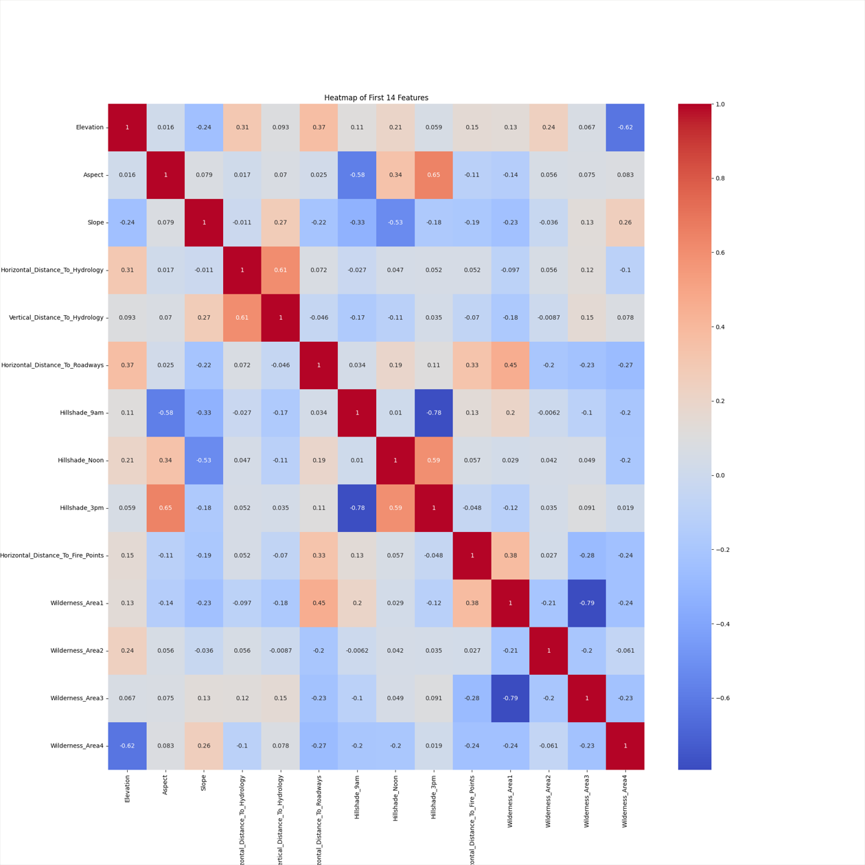
- 训练曲线:
training_curves.png(损失与准确率随 epoch 变化)。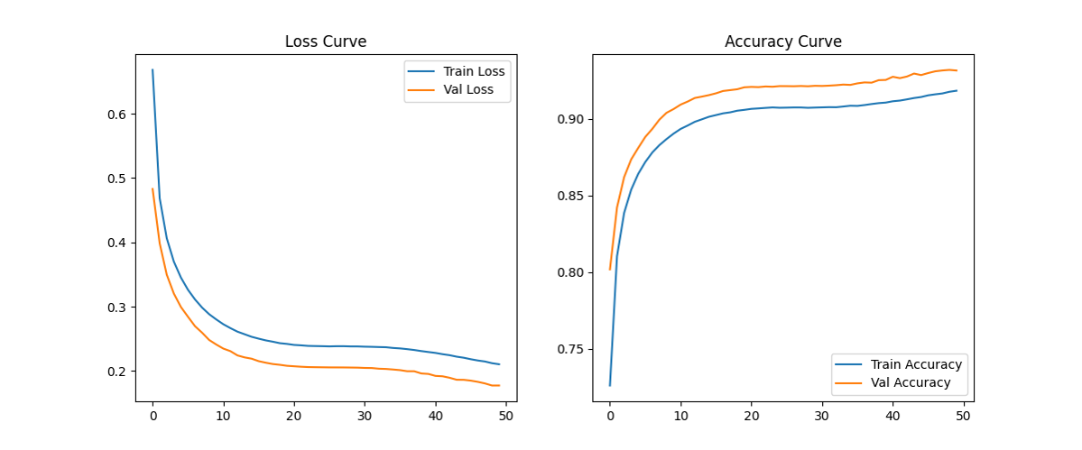
随着epoch的增加,训练和验证的loss逐渐减少,accuracy逐渐增加,最后稳定,模型收敛 特征重要性:
feature_importance.png(随机森林特征排序)。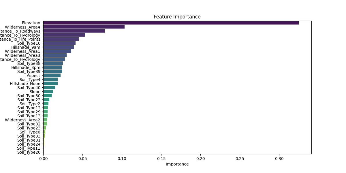
混淆矩阵:
confusion_matrix.png(测试集分类结果热力图)。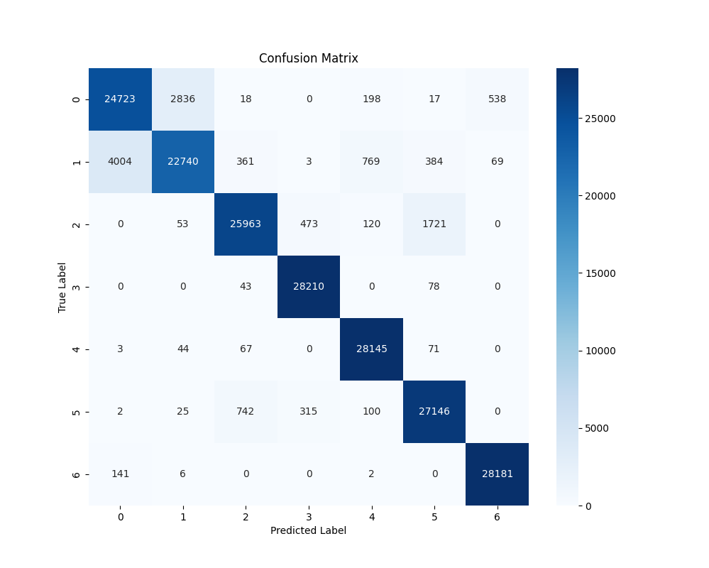
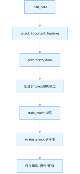
6. 代码执行流程图