群体智能算法解决旅行商问题

实验一 群体智能算法解决旅行商问题

1、实验目的

• 学习蚁群/粒子群/NSGA-II算法在python中的使用与实现；
• 使用蚁群/粒子群/NSGA-II算法解决50个城市的双目标TSP问题；
• 应用多目标决策方法选出最优解（如：TOPSIS）；
• 结果可视化与展示；

2、实验过程

展示主要的建模过程（整体流程+具体修改或完善的地方）文字+图片（如：代码截图）

2.1. A ACO：

代码实现：

graph TD;
    A[开始] --> B[读取数据];
    B --> C[初始化距离和成本矩阵];
    C --> D[初始化参数和信息素];
    D --> E[执行蚁群算法];
    
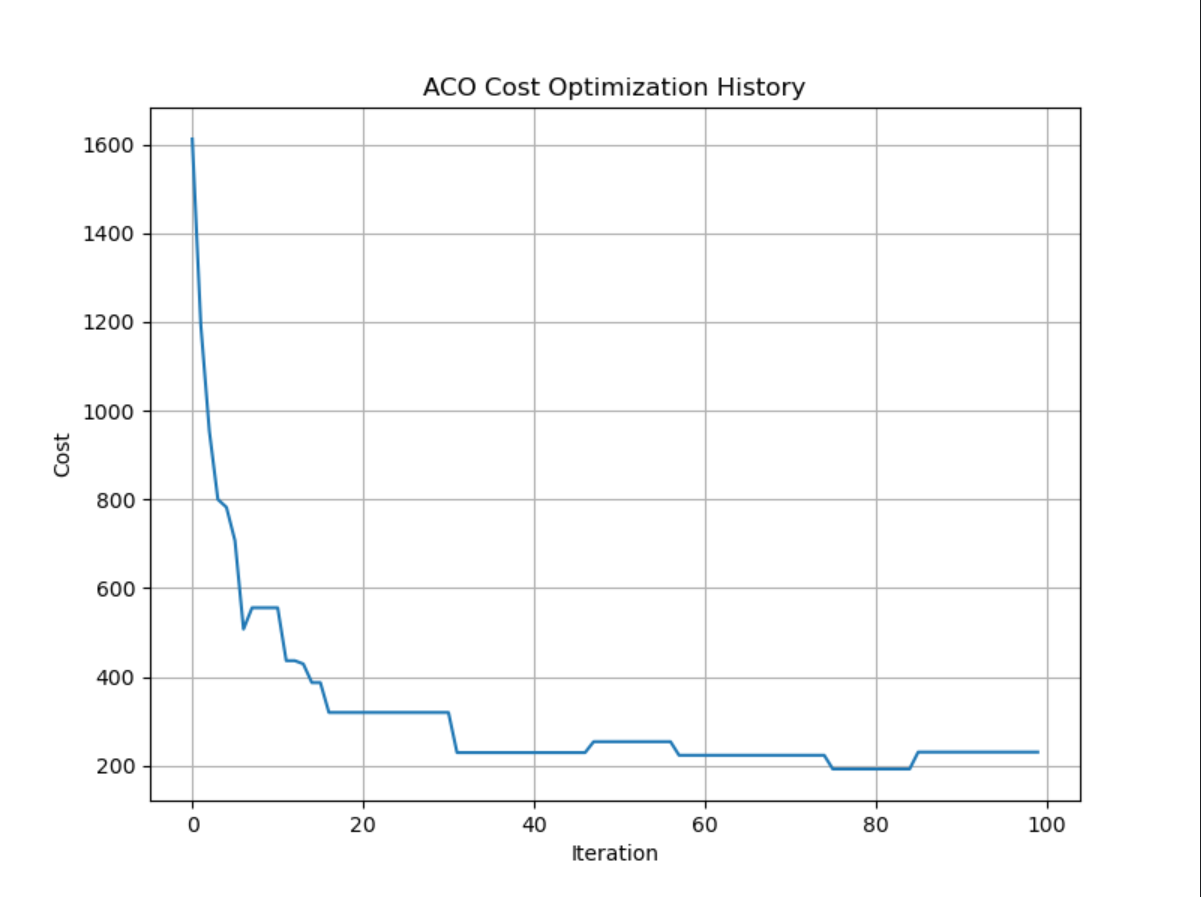
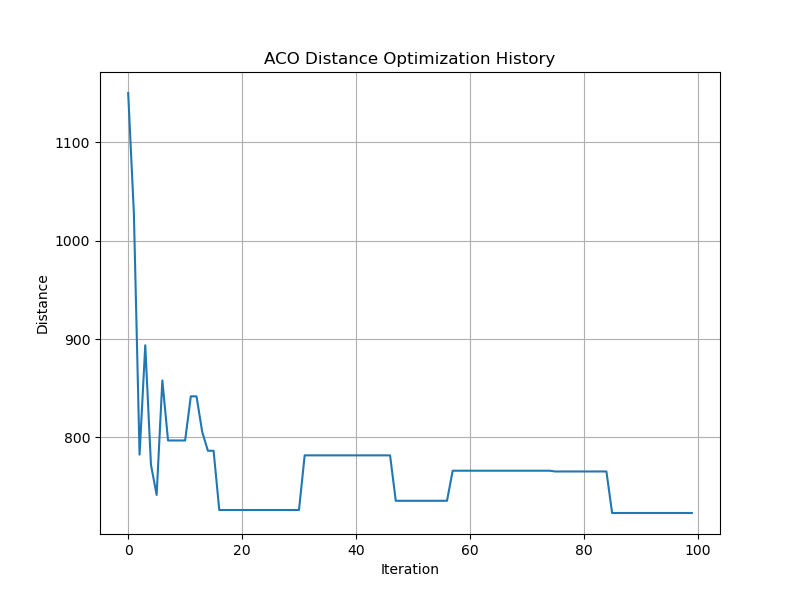
    E --> R[绘制最优路径图];
    E --> S[绘制距离优化图];

    E --> F[构建解决方案];
    F --> G[选择下一个城市];
    G --> H[计算路径长度和成本];
    H --> I[更新信息素];
    I --> J{达到停止条件?};
    J -->|是| K[结束];
    J -->|否| F;

    K --> L[计算最佳解决方案];
    L --> M[输出结果];

    F --> N[检查蚂蚁是否访问所有城市];
    N -->|是| O[添加起始城市到路径];
    N -->|否| G;

    O --> P[计算路径总长度和成本];
    P --> Q[更新最佳解决方案];
    Q --> F;

    
    E --> T[绘制成本优化图];
    E --> U[绘制帕累托前沿图];

import numpy as np
import random
import matplotlib.pyplot as plt
from matplotlib.collections import PolyCollection
import pandas as pd
import math
from tqdm import tqdm
import time

# 读取数据
city_coords = pd.read_excel('city_coordinate.xlsx')
city_costs = pd.read_excel('city_cost.xlsx')

# 辅助函数
def calc_dist(city1, city2):
    """计算两个城市之间的距离"""
    return math.sqrt((city1.iloc[0] - city2.iloc[0]) ** 2 + (city1.iloc[1] - city2.iloc[1]) ** 2)

# 初始化距离矩阵和花费矩阵
dist_matrix = np.zeros((len(city_coords), len(city_coords)))
cost_matrix = np.zeros((len(city_costs), len(city_costs)))

for i in range(len(city_coords)):
    for j in range(len(city_coords)):
        dist_matrix[i][j] = calc_dist(city_coords.iloc[i], city_coords.iloc[j])
        cost_matrix[i][j] = city_costs.iloc[i, j]

# 定义一个计算路径成本的函数
def tour_cost(tour, dist_matrix, cost_matrix):
    total_dist = sum(dist_matrix[tour[i]][tour[(i + 1) % len(tour)]] for i in range(len(tour)))
    total_cost = sum(cost_matrix[tour[i]][tour[(i + 1) % len(tour)]] for i in range(len(tour)))
    return total_dist, total_cost

class AntColonyOptimization:
    def __init__(self, dist_matrix, cost_matrix, num_ants=50, num_iterations=300, alpha=1.0, beta=1.0, q=100, evaporation_rate=0.1):
        self.dist_matrix = dist_matrix
        self.cost_matrix = cost_matrix
        self.num_ants = num_ants
        self.num_iterations = num_iterations
        self.alpha = alpha
        self.beta = beta
        self.q = q
        self.evaporation_rate = evaporation_rate
        self.pheromone = np.ones_like(dist_matrix) / len(dist_matrix)
        self.best_solution = None
        self.best_distance = np.inf
        self.best_cost = np.inf
        self.distance_history = []
        self.cost_history = []
        self.all_solutions = []

    def select_next_city(self, current_city, unvisited_cities):
        pheromones = self.pheromone[current_city][unvisited_cities] ** self.alpha
        heuristic = 1 / (self.dist_matrix[current_city][unvisited_cities] + self.cost_matrix[current_city][unvisited_cities]) ** self.beta
        probabilities = pheromones * heuristic
        probabilities /= probabilities.sum()  # Normalize probabilities
        next_city = np.random.choice(unvisited_cities, p=probabilities)
        return next_city

    def construct_solution(self):
        solutions = []
        for ant in range(self.num_ants):
            current_city = random.randint(0, len(self.dist_matrix) - 1)
            visited_cities = [current_city]
            unvisited_cities = list(set(range(len(self.dist_matrix))) - set([current_city]))

            while unvisited_cities:
                next_city = self.select_next_city(current_city, unvisited_cities)
                visited_cities.append(next_city)
                unvisited_cities.remove(next_city)
                current_city = next_city

            visited_cities.append(visited_cities[0])  # Ensure path is closed
            distance, cost = tour_cost(visited_cities, self.dist_matrix, self.cost_matrix)
            solutions.append((visited_cities, distance, cost))

        return solutions

    def update_pheromone(self, solutions):
        delta_tau = np.zeros_like(self.pheromone)
        best_sol = min(solutions, key=lambda x: x[1] + x[2])
        for sol, dist, cost in solutions:
            for i in range(len(sol) - 1):
                delta_tau[sol[i]][sol[i + 1]] += self.q / (dist + cost)

        # 添加精英保留策略
        for i in range(len(best_sol[0]) - 1):
            delta_tau[best_sol[0][i]][best_sol[0][i + 1]] += self.q / (best_sol[1] + best_sol[2])

        self.pheromone = (1 - self.evaporation_rate) * self.pheromone + delta_tau

    def run(self):
        initial_mutpb = 0.2  # 初始变异率
        final_mutpb = 0.05  # 最终变异率
        initial_cxpb = 0.9  # 初始交叉率
        final_cxpb = 0.5  # 最终交叉率

        for iteration in tqdm(range(self.num_iterations), desc='Running ACO'):
            # 根据进化进度动态调整参数
            progress = iteration / self.num_iterations
            mutpb = initial_mutpb - progress * (initial_mutpb - final_mutpb)
            cxpb = initial_cxpb - progress * (initial_cxpb - final_cxpb)

            solutions = self.construct_solution()
            self.all_solutions.extend(solutions)
            best_sol = min(solutions, key=lambda x: x[1] + x[2])
            if best_sol[1] + best_sol[2] < self.best_distance + self.best_cost:
                self.best_solution = best_sol[0]
                self.best_distance = best_sol[1]
                self.best_cost = best_sol[2]
            self.update_pheromone(solutions)
            self.distance_history.append(self.best_distance)
            self.cost_history.append(self.best_cost)

        return self.best_solution, self.best_distance, self.best_cost

    def plot_solution(self, solution):
        plt.figure(figsize=(8, 6))
        cities_x = [city_coords.iloc[i, 0] for i in solution]
        cities_y = [city_coords.iloc[i, 1] for i in solution]
        plt.plot(cities_x, cities_y, marker='o', linestyle='-')
        # 添加城市编号
        for i, (x, y) in enumerate(zip(cities_x, cities_y)):
            plt.text(x, y, str(i), ha='center', va='bottom', fontsize=8)
        plt.title('ACO Solution')
        plt.xlabel('X')
        plt.ylabel('Y')
        plt.grid(True)
        #保存
        plt.savefig('./aco_result/aco_solution.png')
        plt.show()

    def plot_distance_history(self):
        plt.figure(figsize=(8, 6))
        plt.plot(range(self.num_iterations), self.distance_history)
        plt.title('ACO Distance Optimization History')
        plt.xlabel('Iteration')
        plt.ylabel('Distance')
        plt.grid(True)
        #保存

        plt.savefig('./aco_result/aco_distance_history.png')
        plt.show()

    def plot_cost_history(self):
        plt.figure(figsize=(8, 6))
        plt.plot(range(self.num_iterations), self.cost_history)
        plt.title('ACO Cost Optimization History')
        plt.xlabel('Iteration')
        plt.ylabel('Cost')
        plt.grid(True)
        #保存
        plt.savefig('./aco_result/aco_cost_history.png')
        plt.show()

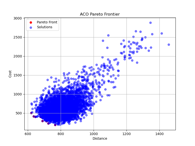
    def plot_pareto_frontier(self):
        distances = [sol[1] for sol in self.all_solutions]
        costs = [sol[2] for sol in self.all_solutions]
        paths = [sol[0] for sol in self.all_solutions]

        pareto_front = []
        pareto_paths = []
        for i in range(len(distances)):
            is_pareto = True
            for j in range(len(distances)):
                if distances[j] < distances[i] and costs[j] < costs[i]:
                    is_pareto = False
                    break
            if is_pareto:
                pareto_front.append((distances[i], costs[i]))
                pareto_paths.append(paths[i])

        pareto_front.sort(key=lambda x: x[0])

        # 保存pareto_front到xlsx,包括路径信息
        df = pd.DataFrame(
            {'Distance': [d for d, c in pareto_front], 'Cost': [c for d, c in pareto_front], 'Path': pareto_paths})
        df.to_excel('./aco_result/aco_pareto_front.xlsx', index=False)

        plt.figure(figsize=(8, 6))
        plt.scatter([d for d, c in pareto_front], [c for d, c in pareto_front], color='r', label='Pareto Front')
        plt.scatter(distances, costs, color='b', label='Solutions', alpha=0.5)
        plt.title('ACO Pareto Frontier')
        plt.xlabel('Distance')
        plt.ylabel('Cost')
        plt.legend()
        plt.grid(True)
        plt.savefig('./aco_result/aco_pareto_frontier.png')
        plt.show()

#if __name__ == '__main__':
def aco_main():
    #开始时间
    start = time.time()

    # 初始化并执行蚁群算法
    aco = AntColonyOptimization(dist_matrix, cost_matrix,num_iterations=100)
    best_path_ACO, best_dist_ACO, best_cost_ACO = aco.run()
    #结束时间
    end = time.time()

    print(f"蚁群算法得到的最优路径: {best_path_ACO}")
    print(f"最短距离: {best_dist_ACO}")
    print(f"最小花费: {best_cost_ACO}")
    
    print('Running time: %s Seconds'%(end-start))

    with open('./aco_result/results.txt', 'w') as file:
        # 写入蚁群算法得到的最优路径
        file.write(f"蚁群算法得到的最优路径: {best_path_ACO}\n")
        # 写入最短距离
        file.write(f"最短距离: {best_dist_ACO}\n")
        # 写入最小花费
        file.write(f"最小花费: {best_cost_ACO}\n")
        file.write('Running time: %s Seconds'%(end-start))

    # 绘制最优路径图
    aco.plot_solution(best_path_ACO)
    # 绘制距离优化图
    aco.plot_distance_history()
    # 绘制花费优化图
    aco.plot_cost_history()
    # 绘制帕累托前沿
    aco.plot_pareto_frontier()
    
aco_main()

2.2. B PSO：

graph TD;
    A[开始] --> B[读取数据];
    B --> C[初始化距离和成本矩阵];
    C --> D[初始化粒子群];
    D --> E[执行粒子群优化算法];

    E --> F[更新粒子位置];
    F --> G[检查个体最优和全局最优];
    G --> H{达到停止条件?};
    H -->|是| I[结束];
    H -->|否| F;

    I --> J[计算最优解];
    J --> K[输出结果];

    F --> L[动态调整参数];
    L --> M[更新信息素];
    M --> F;

    E --> N[绘制最优路径图];
    E --> O[绘制距离优化图];
    E --> P[绘制成本优化图];
    E --> Q[绘制帕累托前沿图];

代码实现：

import numpy as np
import random
import matplotlib.pyplot as plt
import pandas as pd
import math
from tqdm import tqdm
import time

# 读取数据
city_coords = pd.read_excel('city_coordinate.xlsx')
city_costs = pd.read_excel('city_cost.xlsx')

# 辅助函数
def calc_dist(city1, city2):
    """计算两个城市之间的距离"""
    return math.sqrt((city1.iloc[0] - city2.iloc[0]) ** 2 + (city1.iloc[1] - city2.iloc[1]) ** 2)

# 初始化距离矩阵和花费矩阵
dist_matrix = np.zeros((len(city_coords), len(city_coords)))
cost_matrix = np.zeros((len(city_costs), len(city_costs)))

for i in range(len(city_coords)):
    for j in range(len(city_coords)):
        dist_matrix[i][j] = calc_dist(city_coords.iloc[i], city_coords.iloc[j])
        cost_matrix[i][j] = city_costs.iloc[i, j]

# 定义一个计算路径成本的函数
def tour_cost(tour, dist_matrix, cost_matrix):
    """计算给定路径的总距离和总成本"""
    total_dist = sum(dist_matrix[tour[i]][tour[(i + 1) % len(tour)]] for i in range(len(tour)))
    total_cost = sum(cost_matrix[tour[i]][tour[(i + 1) % len(tour)]] for i in range(len(tour)))
    return total_dist, total_cost

class ParticleSwarmOptimization:
    def __init__(self, dist_matrix, cost_matrix, num_particles=50, num_iterations=300, c1=2, c2=2, w=0.9, mutation_rate=0.1, elite_rate=0.1):
        """
        初始化粒子群优化算法的参数
        :param dist_matrix: 距离矩阵
        :param cost_matrix: 成本矩阵
        :param num_particles: 粒子数量
        :param num_iterations: 迭代次数
        :param c1: 个体学习因子
        :param c2: 群体学习因子
        :param w: 惯性权重
        :param mutation_rate: 随机扰动的概率
        :param elite_rate: 精英保留的比例
        """
        self.dist_matrix = dist_matrix
        self.cost_matrix = cost_matrix
        self.num_particles = num_particles
        self.num_iterations = num_iterations
        self.c1 = c1
        self.c2 = c2
        self.w = w
        self.mutation_rate = mutation_rate
        self.elite_rate = elite_rate
        self.particles = []
        self.pbest_positions = []
        self.pbest_distances = []
        self.pbest_costs = []
        self.gbest_position = None
        self.gbest_distance = np.inf
        self.gbest_cost = np.inf
        self.distance_history = []
        self.cost_history = []
        self.all_solutions = []

    def initialize_particles(self):
        """初始化粒子群"""
        for _ in range(self.num_particles):
            particle = random.sample(range(len(self.dist_matrix)), len(self.dist_matrix))
            self.particles.append(particle)
            distance, cost = tour_cost(particle, self.dist_matrix, self.cost_matrix)
            self.pbest_positions.append(particle)
            self.pbest_distances.append(distance)
            self.pbest_costs.append(cost)

            if distance + cost < self.gbest_distance + self.gbest_cost:
                self.gbest_position = particle
                self.gbest_distance = distance
                self.gbest_cost = cost

    def update_particle(self, particle, iteration):
        """更新粒子的位置"""
        new_particle = particle.copy()
        r1 = random.random()
        r2 = random.random()

        # 动态调整参数
        curr_w = self.w * (1 - iteration / self.num_iterations)
        curr_c1 = self.c1 * (1 - iteration / self.num_iterations)
        curr_c2 = self.c2 * (1 - iteration / self.num_iterations)

        for i in range(len(new_particle)):
            # 进行随机扰动
            if random.random() < self.mutation_rate:
                idx1 = random.randint(0, len(new_particle) - 1)
                idx2 = random.randint(0, len(new_particle) - 1)
                new_particle[idx1], new_particle[idx2] = new_particle[idx2], new_particle[idx1]

            distance, cost = tour_cost(new_particle, self.dist_matrix, self.cost_matrix)
            if distance + cost < self.pbest_distances[i] + self.pbest_costs[i]:
                self.pbest_positions[i] = new_particle
                self.pbest_distances[i] = distance
                self.pbest_costs[i] = cost

            if distance + cost < self.gbest_distance + self.gbest_cost:
                self.gbest_position = new_particle
                self.gbest_distance = distance
                self.gbest_cost = cost

        # 精英保留策略
        elite_size = int(self.elite_rate * self.num_particles)
        self.pbest_positions = sorted(self.pbest_positions, key=lambda x: tour_cost(x, self.dist_matrix, self.cost_matrix)[0] + tour_cost(x, self.dist_matrix, self.cost_matrix)[1])[:self.num_particles - elite_size] + self.pbest_positions[:elite_size]
        self.pbest_distances = [tour_cost(p, self.dist_matrix, self.cost_matrix)[0] for p in self.pbest_positions]
        self.pbest_costs = [tour_cost(p, self.dist_matrix, self.cost_matrix)[1] for p in self.pbest_positions]

        return new_particle

    def run(self):
        """运行粒子群优化算法"""
        self.initialize_particles()

        for iteration in tqdm(range(self.num_iterations), desc='Running PSO'):
            new_particles = []
            for particle in self.particles:
                new_particle = self.update_particle(particle, iteration)
                new_particles.append(new_particle)
            self.particles = new_particles

            self.distance_history.append(self.gbest_distance)
            self.cost_history.append(self.gbest_cost)
            self.all_solutions.append((self.gbest_position, self.gbest_distance, self.gbest_cost))

        return self.gbest_position, self.gbest_distance, self.gbest_cost

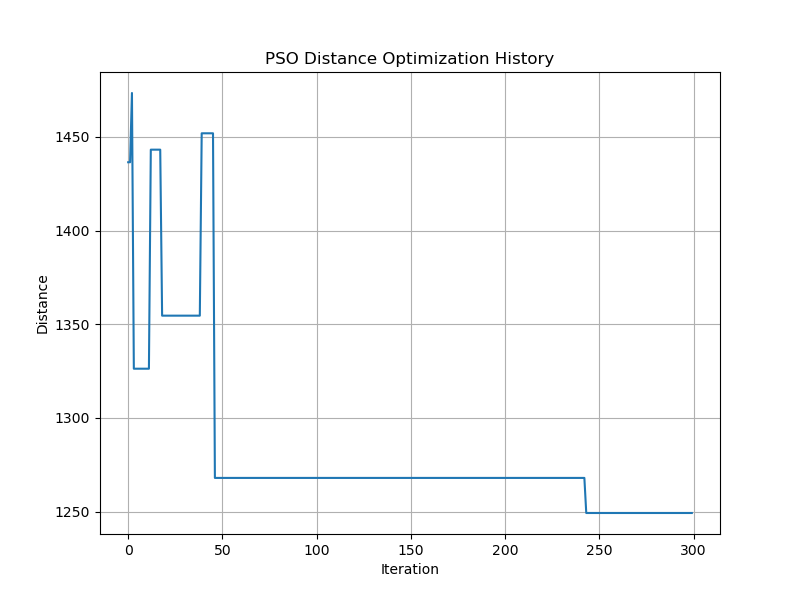
    def plot_solution(self, solution):
        """绘制最优路径图"""
        plt.figure(figsize=(8, 6))
        cities_x = [city_coords.iloc[i, 0] for i in solution]
        cities_y = [city_coords.iloc[i, 1] for i in solution]
        plt.plot(cities_x, cities_y, marker='o', linestyle='-')

        # 添加城市编号
        for i, (x, y) in enumerate(zip(cities_x, cities_y)):
            plt.text(x, y, str(i), ha='center', va='bottom', fontsize=8)

        plt.title('PSO Solution')
        plt.xlabel('X')
        plt.ylabel('Y')
        plt.grid(True)
        plt.savefig('./pso_result/pso_solution.png')
        plt.show()

    def plot_distance_history(self):
        """绘制距离优化历史图"""
        plt.figure(figsize=(8, 6))
        plt.plot(range(self.num_iterations), self.distance_history)
        plt.title('PSO Distance Optimization History')
        plt.xlabel('Iteration')
        plt.ylabel('Distance')
        plt.grid(True)
        plt.savefig('./pso_result/pso_distance_history.png')
        plt.show()

    def plot_cost_history(self):
        """绘制成本优化历史图"""
        plt.figure(figsize=(8, 6))
        plt.plot(range(self.num_iterations), self.cost_history)
        plt.title('PSO Cost Optimization History')
        plt.xlabel('Iteration')
        plt.ylabel('Cost')
        plt.grid(True)
        plt.savefig('./pso_result/pso_cost_history.png')
        plt.show()

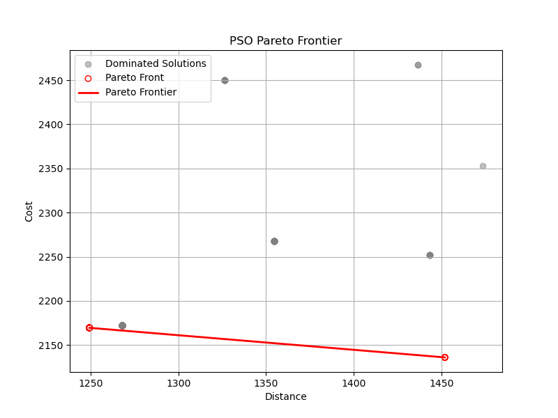
    def plot_pareto_frontier(self):
        """绘制帕累托前沿图并保存数据"""
        distances = [sol[1] for sol in self.all_solutions]
        costs = [sol[2] for sol in self.all_solutions]
        tours = [sol[0] for sol in self.all_solutions]

        pareto_front = []
        pareto_tours = []
        dominated_solutions = []

        for i in range(len(distances)):
            is_pareto = True
            for j in range(len(distances)):
                if distances[j] < distances[i] and costs[j] < costs[i]:
                    is_pareto = False
                    break
            if is_pareto:
                pareto_front.append((distances[i], costs[i]))
                pareto_tours.append(tours[i])
            else:
                dominated_solutions.append((distances[i], costs[i], tours[i]))

        pareto_front = sorted(pareto_front, key=lambda x: x[0])
        pareto_tours = [pareto_tours[i] for i in sorted(range(len(pareto_front)), key=lambda k: pareto_front[k][0])]

        # 将帕累托前沿数据保存到 Excel 文件
        df = pd.DataFrame({
            'Distance': [d for d, c in pareto_front],
            'Cost': [c for d, c in pareto_front],
            'Path': pareto_tours
        })
        df.to_excel('./pso_result/pso_pareto_front.xlsx', index=False)

        plt.figure(figsize=(8, 6))
        plt.scatter([d for d, c, _ in dominated_solutions], [c for d, c, _ in dominated_solutions], color='gray',
                    label='Dominated Solutions', alpha=0.5)
        plt.scatter([d for d, c in pareto_front], [c for d, c in pareto_front], color='r', label='Pareto Front',
                    marker='o', facecolors='none')
        plt.plot([d for d, c in pareto_front], [c for d, c in pareto_front], color='r', label='Pareto Frontier',
                 linewidth=2)
        plt.title('PSO Pareto Frontier')
        plt.xlabel('Distance')
        plt.ylabel('Cost')
        plt.legend()
        plt.grid(True)
        plt.savefig('./pso_result/pso_pareto_frontier.png')
        plt.show()

def pso_main():
    """主函数,运行粒子群优化算法"""
    start = time.time()
    pso = ParticleSwarmOptimization(dist_matrix, cost_matrix, num_iterations=300, mutation_rate=0.1, elite_rate=0.1)
    best_path_PSO, best_dist_PSO, best_cost_PSO = pso.run()
    end = time.time()

    print(f"粒子群算法得到的最优路径: {best_path_PSO}")
    print(f"最短距离: {best_dist_PSO}")
    print(f"最小花费: {best_cost_PSO}")
    print('Running time: %s Seconds'%(end-start))

    with open('./pso_result/results.txt', 'w') as file:
        # 写入蚁群算法得到的最优路径
        file.write(f"粒子群算法得到的最优路径: {best_path_PSO}\n")
        # 写入最短距离
        file.write(f"最短距离: {best_dist_PSO}\n")
        # 写入最小花费
        file.write(f"最小花费: {best_cost_PSO}\n")
        file.write('Running time: %s Seconds'%(end-start))

    pso.plot_solution(best_path_PSO)
    pso.plot_distance_history()
    pso.plot_cost_history()
    pso.plot_pareto_frontier()

pso_main()

2.3. C NSGA-II：

代码实现：

graph TD;
    A[开始] --> B[读取数据];
    B --> C[创建 TSP 实例];
    C --> D[运行 NSGA2 优化器];
    D --> E{是否达到最大代数?};
    E -->|是| F[结束];
    E -->|否| G[选择];
    G --> H[交叉和变异];
    H --> I[评估子代];
    I --> J[选择下一代];
    J --> E;

    F --> K[获取帕累托前沿];
    K --> L[保存到 Excel];
    L --> M[查找最小距离和最小成本解];
    M --> N[打印绘制结果];

import numpy as np
import random
import matplotlib.pyplot as plt
from deap import base, creator, tools, algorithms
import pandas as pd
import math
from tqdm import tqdm
import time

class TravelingSalesmanProblem:
    def __init__(self, city_coords, city_costs):
        self.city_coords = city_coords
        self.city_costs = city_costs
        self.num_cities = len(city_coords)
        self.dist_matrix = self._calculate_distance_matrix()
        self.cost_matrix = self._calculate_cost_matrix()

    def _calculate_distance_matrix(self):
        dist_matrix = np.zeros((self.num_cities, self.num_cities))
        for i in range(self.num_cities):
            for j in range(self.num_cities):
                dist_matrix[i][j] = self._calculate_distance(self.city_coords.iloc[i], self.city_coords.iloc[j])
        return dist_matrix

    def _calculate_cost_matrix(self):
        cost_matrix = np.zeros((self.num_cities, self.num_cities))
        for i in range(self.num_cities):
            for j in range(self.num_cities):
                cost_matrix[i][j] = self.city_costs.iloc[i, j]
        return cost_matrix

    def _calculate_distance(self, city1, city2):
        return math.sqrt((city1['X'] - city2['X']) ** 2 + (city1['Y'] - city2['Y']) ** 2)

    def evaluate_individual(self, individual):
        total_distance = 0
        total_cost = 0
        for i in range(len(individual)):
            if i == len(individual) - 1:
                total_distance += self.dist_matrix[individual[i]][individual[0]]
                total_cost += self.cost_matrix[individual[i]][individual[0]]
            else:
                total_distance += self.dist_matrix[individual[i]][individual[i + 1]]
                total_cost += self.cost_matrix[individual[i]][individual[i + 1]]
        return total_distance, total_cost

class NSGA2Optimizer:
    def __init__(self, tsp, pop_size, max_gen, cxpb, mutpb):
        self.tsp = tsp
        self.pop_size = pop_size
        self.max_gen = max_gen
        self.cxpb = cxpb
        self.mutpb = mutpb
        self.min_distances = []
        self.min_costs = []

        # Define problem objectives
        creator.create("FitnessMulti", base.Fitness, weights=(-1.0, -1.0))
        creator.create("Individual", list, fitness=creator.FitnessMulti)

        # Define toolbox
        self.toolbox = base.Toolbox()
        self.toolbox.register("attribute", lambda: [random.randint(0, self.tsp.num_cities - 1) for _ in range(self.tsp.num_cities)])
        self.toolbox.register("individual", tools.initIterate, creator.Individual, self.toolbox.attribute)
        self.toolbox.register("population", tools.initRepeat, list, self.toolbox.individual)
        self.toolbox.register("evaluate", self.tsp.evaluate_individual)
        self.toolbox.register("select", tools.selNSGA2)
        self.toolbox.register("mate", tools.cxPartialyMatched)
        self.toolbox.register("mutate", tools.mutShuffleIndexes, indpb=1.0 / self.tsp.num_cities)

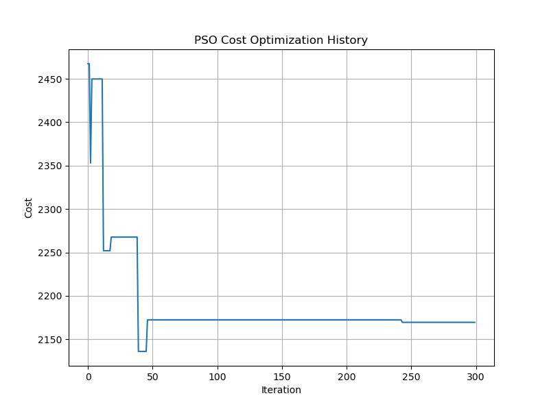
    def run(self):
        # Initialize population
        pop = self.toolbox.population(n=self.pop_size)

        # Evaluate initial population
        fitnesses = list(map(self.toolbox.evaluate, pop))
        for ind, fit in zip(pop, fitnesses):
            ind.fitness.values = fit

        # Evolution loop
        for g in tqdm(range(self.max_gen), desc="Running NSGA"):
            # Selection
            offspring = self.toolbox.select(pop, len(pop))

            # Crossover and mutation
            offspring = [self.toolbox.clone(ind) for ind in offspring]
            for i in range(1, len(offspring), 2):
                if random.random() < self.cxpb:
                    self.toolbox.mate(offspring[i - 1], offspring[i])
                    del offspring[i - 1].fitness.values, offspring[i].fitness.values

            for mutant in offspring:
                if random.random() < self.mutpb:
                    self.toolbox.mutate(mutant)
                    del mutant.fitness.values

            # Evaluate offspring
            invalid_ind = [ind for ind in offspring if not ind.fitness.valid]
            fitnesses = map(self.toolbox.evaluate, invalid_ind)
            for ind, fit in zip(invalid_ind, fitnesses):
                ind.fitness.values = fit

            # Select the next generation
            pop = self.toolbox.select(pop + offspring, self.pop_size)

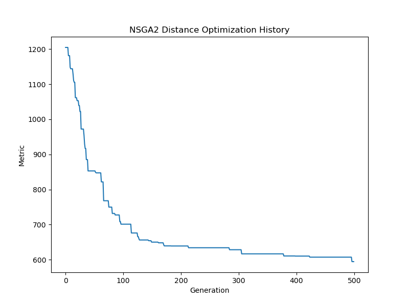
            # Update minimum distance and minimum cost
            self.min_distances.append(min(ind.fitness.values[0] for ind in pop))
            self.min_costs.append(min(ind.fitness.values[1] for ind in pop))

        return pop

def nsga_main():
    # Start time
    start_time = time.time()

    # Read data
    city_coords = pd.read_excel('city_coordinate.xlsx')
    city_costs = pd.read_excel('city_cost.xlsx')

    # Create TSP instance
    tsp = TravelingSalesmanProblem(city_coords, city_costs)

    # Run NSGA2 optimizer
    nsga2 = NSGA2Optimizer(tsp, pop_size=100, max_gen=500, cxpb=0.8, mutpb=0.2)
    final_pop = nsga2.run()

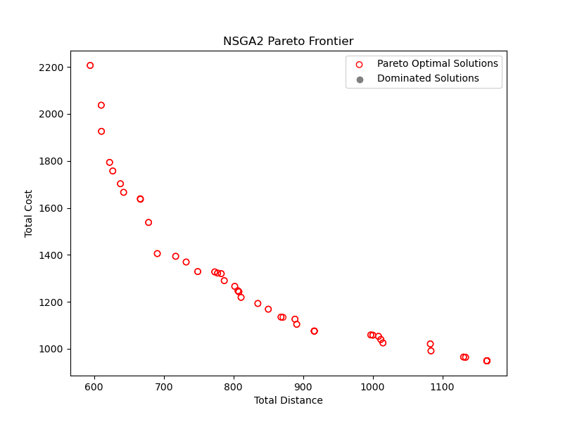
    # Get Pareto front
    pareto_front = tools.emo.sortNondominated(final_pop, len(final_pop))

    # Create a list to store the Pareto front data
    pareto_front_data = []

    # Iterate through the Pareto front and collect the data
    for individual in pareto_front[0]:
        distance, cost = tsp.evaluate_individual(individual)
        pareto_front_data.append((distance, cost, individual))

    # Convert the data to a pandas DataFrame and save to Excel
    pareto_front_df = pd.DataFrame(pareto_front_data, columns=['Distance', 'Cost', 'Path'])
    pareto_front_df.to_excel('./nsga2_result/nsga_pareto_front.xlsx', index=False)

    # Find minimum distance and minimum cost solutions
    min_distance_ind, min_distance = find_minimum_solution(tsp, pareto_front[0], 'distance')
    min_cost_ind, min_cost = find_minimum_solution(tsp, pareto_front[0], 'cost')

    # End time
    end_time = time.time()
    print(f"Execution time: {end_time - start_time:.2f} seconds")
    with open('./nsga2_result/results.txt', 'w') as file:
        file.write(f"Execution time: {end_time - start_time:.2f} seconds\n")

    # Print results
    print_results(min_distance_ind, min_distance, min_cost_ind, min_cost)

    # Plot results
    plot_results(tsp, min_distance_ind, final_pop, pareto_front, nsga2)

def find_minimum_solution(tsp, pareto_front, objective):
    if objective == 'distance':
        min_value = float('inf')
        min_individual = None
    elif objective == 'cost':
        min_value = float('inf')
        min_individual = None
    else:
        raise ValueError("Invalid objective. Choose 'distance' or 'cost'.")

    for individual in pareto_front:
        total_value = tsp.evaluate_individual(individual)[['distance', 'cost'].index(objective)]
        if total_value < min_value:
            min_value = total_value
            min_individual = individual

    return min_individual, min_value

def print_results(min_distance_ind, min_distance, min_cost_ind, min_cost):
    print(f"Minimum Distance Route: {min_distance_ind}")
    print(f"Minimum Distance: {min_distance:.2f}")
    print()
    print(f"Minimum Cost Route: {min_cost_ind}")
    print(f"Minimum Cost: {min_cost:.2f}")

    with open('./nsga2_result/results.txt', 'a') as file:
        file.write(f"Minimum Distance Route: {min_distance_ind}\n")
        file.write(f"Minimum Distance: {min_distance:.2f}\n")
        file.write(f"Minimum Cost Route: {min_cost_ind}\n")
        file.write(f"Minimum Cost: {min_cost:.2f}\n")

def plot_results(tsp, min_distance_ind, final_pop, pareto_front, nsga2):
    # Plot minimum distance route
    plot_route(tsp, min_distance_ind, './nsga2_result/nsga2_solution.png', 'NSGA2 Solution')

    # Plot Pareto frontier
    plot_pareto_frontier(final_pop, pareto_front, './nsga2_result/nsga2_pareto_frontier.png', 'NSGA2 Pareto Frontier')

    # Plot minimum distance optimization history
    plot_optimization_history(nsga2.min_distances, './nsga2_result/nsga2_distance_history.png', 'NSGA2 Distance Optimization History')

    # Plot minimum cost optimization history
    plot_optimization_history(nsga2.min_costs, './nsga2_result/nsga2_cost_history.png', 'NSGA2 Cost Optimization History')

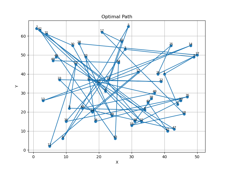
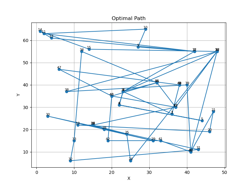
def plot_route(tsp, route, save_path, title):
    plt.figure(figsize=(8, 6))
    route_x = [tsp.city_coords.iloc[city]['X'] for city in route]
    route_y = [tsp.city_coords.iloc[city]['Y'] for city in route]
    route_x.append(route_x[0])  # Close the loop
    route_y.append(route_y[0])  # Close the loop
    plt.plot(route_x, route_y, '-o')
    for i, city in enumerate(route):
        plt.text(tsp.city_coords.iloc[city]['X'], tsp.city_coords.iloc[city]['Y'], str(city), fontsize=8)
    plt.xlabel('X Coordinate')
    plt.ylabel('Y Coordinate')
    plt.title(title)
    plt.savefig(save_path)
    plt.show()

def plot_pareto_frontier(final_pop, pareto_front, save_path, title):
    plt.figure(figsize=(8, 6))

    # Plot Pareto front
    distances = [ind.fitness.values[0] for ind in pareto_front[0]]
    costs = [ind.fitness.values[1] for ind in pareto_front[0]]
    #plt.plot(distances, costs, '-r', label='Pareto Front')

    # Plot Pareto optimal solutions
    pareto_distances = [ind.fitness.values[0] for ind in pareto_front[0]]
    pareto_costs = [ind.fitness.values[1] for ind in pareto_front[0]]
    plt.scatter(pareto_distances, pareto_costs, facecolors='none', edgecolors='r', label='Pareto Optimal Solutions')

    # Plot dominated solutions
    dominated_distances = [ind.fitness.values[0] for ind in final_pop if ind not in pareto_front[0]]
    dominated_costs = [ind.fitness.values[1] for ind in final_pop if ind not in pareto_front[0]]
    plt.scatter(dominated_distances, dominated_costs, color='gray', label='Dominated Solutions')

    plt.xlabel('Total Distance')
    plt.ylabel('Total Cost')
    plt.title(title)
    plt.legend()
    plt.savefig(save_path)
    plt.show()

def plot_optimization_history(history, save_path, title):
    plt.figure(figsize=(8, 6))
    plt.plot(range(len(history)), history)
    plt.xlabel('Generation')
    plt.ylabel('Metric')
    plt.title(title)
    plt.savefig(save_path)
    plt.show()

nsga_main()

2.4. D 多目标问题决策（topsis)：

graph TD;
    A[读取 city_coordinate.xlsx] --> B[Normalization1 和 EntropyWeight 计算];
    B --> C[TOPSIS 分析];
    C --> D[输出 ACO 的最优解];
    C --> E[输出 PSO 的最优解];
    C --> F[输出 NSGA2 的最优解];
    D --> G[绘制 ACO 的最优路径图];
    E --> H[绘制 PSO 的最优路径图];
    F --> I[绘制 NSGA2 的最优路径图];

import pandas as pd  
import numpy as np  
import matplotlib.pyplot as plt  
import sys  
  
# 重定向stdout到文件  
orig_stdout = sys.stdout  
f = open('output.txt', 'w')  
sys.stdout = f  
  
city_coords = pd.read_excel('city_coordinate.xlsx')  
  
# Normalization and Entropy Weight Functions  
def normalization1(data):  
    _range = np.max(data) - np.min(data)  
    return (data - np.min(data)) / _range  
  
def entropyWeight(data):  
    P = np.array(data)  
    P[P == 0] = 1e-10  
    E = np.nansum(-P * np.log(P) / np.log(len(data)), axis=0)  
    return (1 - E) / (1 - E).sum()  
  
# TOPSIS Function  
def topsis(data, weight=None):  
    weight = entropyWeight(data) if weight is None else np.array(weight)  
    Z = pd.DataFrame([(data * weight.T).min(), (data * weight.T).max()], index=['负理想解', '正理想解'])  
    Result = data.copy()  
    Result['正理想解'] = np.sqrt(((data - Z.loc['正理想解']) ** 2).sum(axis=1))  
    Result['负理想解'] = np.sqrt(((data - Z.loc['负理想解']) ** 2).sum(axis=1))  
    Result['综合得分指数'] = Result['负理想解'] / (Result['负理想解'] + Result['正理想解'])  
    Result['排序'] = Result.rank(ascending=False)['综合得分指数']  
    return Result, Z, weight  
  
# Analysis Function  
def analysis(file_path):  
    data = pd.read_excel(file_path)  
    data1 = data.copy()  
    data1 = data1.drop(columns=['Path'])  
    data1['Distance'] = normalization1(data1['Distance'])  
    data1['Cost'] = normalization1(data1['Cost'])  
    [result, z1, weight] = topsis(data1)  
    best_solution_index = result['排序'].idxmin()  
    best_solution_data = data.loc[best_solution_index]  
    print("最优解的原数据:")  
    print(best_solution_data)  
    optimal_path = [int(x) for x in best_solution_data['Path'].strip('[]').split(', ')]  
    return optimal_path  
  
# Plot Solution Function  
def plot_solution(optimal_path, file_name):  
    plt.figure(figsize=(8, 6))  
    cities_x = [city_coords.iloc[i, 0] for i in optimal_path]  
    cities_y = [city_coords.iloc[i, 1] for i in optimal_path]  
    plt.plot(cities_x, cities_y, marker='o', linestyle='-')  
  
    for i, (x, y) in enumerate(zip(cities_x, cities_y)):  
        plt.text(x, y, str(i), ha='center', va='bottom', fontsize=8)  
  
    plt.title('Optimal Path')  
    plt.xlabel('X')  
    plt.ylabel('Y')  
    plt.grid(True)  
    #plt.savefig(file_name)  
    plt.show()  
  
if __name__ == '__main__':  
    print("ACO Pareto Front Analysis:")  
    aco_optimal_path = analysis('./aco_result/aco_pareto_front.xlsx')  
    print("PSO Pareto Front Analysis:")  
    pso_optimal_path = analysis('./pso_result/pso_pareto_front.xlsx')  
    print("NSGA2 Pareto Front Analysis:")  
    nsga2_optimal_path = analysis('./nsga2_result/nsga_pareto_front.xlsx')  
  
    print("ACO optimal path:", aco_optimal_path)  
    print("PSO optimal path:", pso_optimal_path)  
    print("NSGA2 optimal path:", nsga2_optimal_path)  
  
    plot_solution(aco_optimal_path, './aco_result/aco_solution.png')  
    plot_solution(pso_optimal_path, './pso_result/pso_solution.png')  
    plot_solution(nsga2_optimal_path, './nsga2_result/nsga2_solution.png')  
  
    # 恢复stdout  
    sys.stdout = orig_stdout  
    f.close()

结果：

ACO Pareto Front Analysis:
最优解的原数据:
Distance                                            723.22809
Cost                                               230.172644
Path        [20, 25, 26, 27, 28, 1, 5, 6, 7, 8, 9, 10, 23,...
Name: 8, dtype: object
PSO Pareto Front Analysis:
最优解的原数据:
Distance                                          1249.282921
Cost                                              2169.537487
Path        [43, 39, 48, 27, 8, 28, 21, 0, 33, 10, 12, 4, ...
Name: 0, dtype: object
NSGA2 Pareto Front Analysis:
最优解的原数据:
Distance                                           782.507764
Cost                                              1320.000846
Path        [37, 35, 35, 22, 21, 43, 21, 22, 41, 26, 28, 1...
Name: 86, dtype: object
ACO optimal path: [20, 25, 26, 27, 28, 1, 5, 6, 7, 8, 9, 10, 23, 24, 29, 30, 31, 37, 38, 39, 40, 32, 33, 34, 35, 36, 4, 2, 14, 42, 43, 44, 45, 46, 47, 48, 49, 41, 3, 0, 21, 22, 11, 12, 13, 15, 16, 17, 18, 19, 20]
PSO optimal path: [43, 39, 48, 27, 8, 28, 21, 0, 33, 10, 12, 4, 31, 2, 47, 22, 26, 20, 45, 29, 44, 16, 38, 7, 17, 41, 37, 49, 13, 23, 11, 3, 32, 15, 18, 46, 9, 19, 30, 35, 34, 40, 1, 24, 25, 5, 6, 42, 14, 36]
NSGA2 optimal path: [37, 35, 35, 22, 21, 43, 21, 22, 41, 26, 28, 1, 41, 3, 0, 13, 47, 36, 14, 10, 45, 46, 40, 47, 24, 23, 14, 14, 17, 30, 2, 42, 8, 9, 11, 31, 22, 47, 7, 39, 40, 32, 18, 19, 31, 36, 19, 5, 37, 37]

2.5. E 三种算法结果比较：

在这里分别对每个算法尝试了10次，选取最优的结果如下：

2.5.1. ACO

蚁群算法得到的最优路径: [3, 0, 1, 5, 6, 7, 8, 9, 10, 11, 12, 13, 15, 16, 17, 18, 19, 20, 21, 22, 25, 26, 27, 28, 4, 2, 14, 33, 34, 35, 36, 37, 38, 39, 40, 32, 23, 24, 29, 30, 31, 41, 42, 43, 44, 45, 46, 47, 48, 49, 3]  
最短距离: 723.2280896516359  
最小花费: 230.17264374788454  
Running time: 11.859421253204346 Seconds

2.5.2. PSO

粒子群算法得到的最优路径: [0, 29, 39, 16, 4, 47, 30, 19, 26, 18, 2, 12, 49, 31, 21, 14, 10, 8, 13, 28, 15, 22, 42, 44, 43, 9, 36, 40, 37, 5, 6, 3, 32, 23, 24, 45, 1, 7, 20, 41, 38, 27, 25, 35, 34, 17, 33, 48, 46, 11]  
最短距离: 1249.2829212381564  
最小花费: 2169.5374873285705  
Running time: 170.3362991809845 Seconds

2.5.3. NSGA-II

Execution time: 8.38 seconds  
Minimum Distance Route: [35, 35, 37, 31, 43, 21, 21, 11, 41, 26, 28, 1, 41, 3, 0, 13, 47, 14, 14, 10, 45, 46, 17, 30, 24, 23, 14, 36, 36, 36, 2, 31, 26, 22, 22, 19, 40, 42, 7, 39, 36, 18, 18, 8, 9, 32, 19, 5, 37, 37]  
Minimum Distance: 594.36  
Minimum Cost Route: [35, 35, 40, 2, 21, 43, 42, 40, 41, 26, 28, 1, 2, 0, 3, 13, 47, 36, 14, 10, 45, 46, 47, 36, 37, 24, 14, 14, 22, 23, 30, 21, 22, 9, 11, 7, 8, 36, 19, 39, 40, 32, 18, 19, 41, 17, 31, 5, 37, 37]  
Minimum Cost: 948.99

3、结果展示

3.1. A ACO：

3.1.1. (1) 运行结果：

迭代优化的过程图

3.1.2. (2) 多目标优化结果：

Pareto图

选择最优解方法的结果（如：TOPSIS分值）

3.1.3. (3) 最优路径：

最优路径图

3.2. B PSO：

3.2.1. (1) 运行结果：

迭代优化的过程图

0.3.2.2. (2) 多目标优化结果：

Pareto图
选择最优解方法的结果（如：TOPSIS分值）

0.3.2.3. (3) 最优路径：

3.3. C NSGA-II：

3.3.1. (1) 运行结果：

迭代优化的过程图

3.3.2. (2) 多目标优化结果：

Pareto图
选择最优解方法的结果（如：TOPSIS分值）

3.3.3. (3) 最优路径：

最优路径图

3.4. D 三种算法结果比较：

指标对比表格

	最小花费	最短距离	TOPSIS优化后的最优路径
ACO	230.17264374788454	723.2280896516359	[20, 25, 26, 27, 28, 1, 5, 6, 7, 8, 9, 10, 23, 24, 29, 30, 31, 37, 38, 39, 40, 32, 33, 34, 35, 36, 4, 2, 14, 42, 43, 44, 45, 46, 47, 48, 49, 41, 3, 0, 21, 22, 11, 12, 13, 15, 16, 17, 18, 19, 20]
PSO	2169.5374873285705	1249.2829212381564	[43, 39, 48, 27, 8, 28, 21, 0, 33, 10, 12, 4, 31, 2, 47, 22, 26, 20, 45, 29, 44, 16, 38, 7, 17, 41, 37, 49, 13, 23, 11, 3, 32, 15, 18, 46, 9, 19, 30, 35, 34, 40, 1, 24, 25, 5, 6, 42, 14, 36]
NSGA-II	948.99	594.36	[37, 35, 35, 22, 21, 43, 21, 22, 41, 26, 28, 1, 41, 3, 0, 13, 47, 36, 14, 10, 45, 46, 40, 47, 24, 23, 14, 14, 17, 30, 2, 42, 8, 9, 11, 31, 22, 47, 7, 39, 40, 32, 18, 19, 31, 36, 19, 5, 37, 37]

通过上面表格比较可知。蚁群算法和遗传算法较粒子群算法效果更优，当然这里并没有考虑算法的运行时间等其他因素。